Baseline regression
Classical baseline correction subtracts the mean of a pre-stimulus window from each epoch. This assumes the baseline is pure noise - but if the baseline co-varies with the epoch (through slow drifts, noise correlations, or the overlap of the previous trial), correcting removes that shared variance from the whole epoch and can bias the estimated effects.
Baseline regression (Alday et al., 2021) instead treats the baseline as a predictor: it is entered into the model as a channel-varying covariate, because the baseline amplitude differs per channel. In Unfold.jl, channel-varying predictors are marked with bychannel: the model is fit per channel, with each channel's epochs regressed on its own baseline. No data is subtracted - the bsl coefficient tells you how strongly the epoch co-varies with the baseline at every latency.
Set things up
using Unfold
using UnfoldSim
using UnfoldMakie
using DataFrames
using Statistics
using Random
Simulate data with a slow drift
We simulate multichannel EEG with UnfoldSim.jl - deliberately with only 200 events and little noise - and add a slow drift to the signal: exponentially correlated noise (ExponentialNoise) with channel-specific amplitude. We also present the two conditions in blocks (event_order_function), so each condition is recorded against a different level of the drift - like a real block experiment where the environment changes over the session. The simulation projects the components onto all 227 channels; for this tutorial we keep three example channels:
data, evts = UnfoldSim.predef_eeg(;
    multichannel = true, n_repeats = 10, overlap = (2, 0.2), noiselevel = 0.1,
    event_order_function = (rng, x) -> sort(x, :condition),
)
data = data[[130, 184, 50], :]

sfreq = 100
amps = [5.0, 4.0, 3.0]
rng = MersenneTwister(1)Random.MersenneTwister(1)τ = 250 samples = 2.5 s: comparable to the 1.7 s epochs, so the drift varies within the epoch
for ch in 1:3
    data[ch, :] .+= simulate_noise(
        rng, ExponentialNoise(noiselevel = amps[ch], τ = 250), size(data, 2),
    )
end
We drop the last events, whose epochs would run past the end of the recording, and cut the continuous data into epochs:
evts = evts[evts.latency .<= size(data, 2) - 150, :]
data_e, times = Unfold.epoch(data = data, tbl = evts, τ = (-0.2, 1.5), sfreq = sfreq)
(Union{Missing, Float64}[1.0941305018450374 1.4580443133681866 … 0.6467660081120606 -0.1777536637326742; 2.178818753342009 1.96151157497061 … 3.9093100711760544 4.493047696865113; -1.1570519129783656 -1.155508523799939 … -5.732109967930103 -5.437597812482808;;; 0.4544925301921666 1.235064501776596 … 2.3273350205510526 1.8056106977768733; 5.109568879564434 5.004597208641829 … 3.531441657735804 3.939857421827286; -5.869059697953722 -5.634639168710903 … 0.2792288469089013 0.8635328293883697;;; 1.8802699332520376 1.4011253895145637 … 1.0077200331418303 0.9394070273197188; 3.214287008904545 3.9870147802563602 … 6.742337788183264 6.308218742954882; -3.4739152038018393 -3.626622291700864 … -5.353927537143923 -5.035360405851539;;; … ;;; 0.9201800935722 0.9351707721357374 … 5.652519250321435 5.803535794951701; -0.26606989664391545 -0.42204106121515333 … 0.4899495125940431 -0.10685419413297208; -3.780580350201647 -3.7346318069147086 … -3.2160554907893446 -3.3554877542169943;;; 6.956979131080679 6.160269201723174 … 9.622411909226761 9.33310421168046; -2.39302162758254 -2.620385056494267 … -9.23894932343914 -9.067000576801185; -1.4540824803305632 -0.7367177597607547 … -1.5995091075874426 -1.465319503307191;;; 10.874066978072783 10.742882378666312 … 9.193121702891878 8.496865183225777; -7.294483713502867 -7.517706945426227 … -5.591177760942218 -5.363280431792537; -4.273099262566426 -4.234804603038828 … -1.3843069781032333 -1.0821155645407186], -0.2:0.01:1.5)Baseline regression
For each channel and epoch, we compute the mean baseline and enter it into the event table as one value per channel per row:
bsl_ix = findall(t -> t <= 0.0, times)
evts.bsl = [vec(mean(data_e[:, bsl_ix, i]; dims = 2)) for i in axes(data_e, 3)]
199-element Vector{Vector{Union{Missing, Float64}}}:
[0.026752598037190555, 1.4280187800073452, -2.4064557492626233]
[1.4744681053083826, 4.873151579878443, -5.039111952624391]
[1.3982614982988402, 4.627721890285441, -3.9353960397261405]
[3.2838884667010553, 3.370920775832568, -3.0511463547689495]
[4.529727329995292, -4.04797923848124, 0.7415657032163785]
[4.682651465683289, 2.889380252928728, -1.1492533419087632]
[7.91485825192235, 0.17067065803549916, 0.9119436845914807]
[-2.377045228176146, -1.8837767807361694, 2.085601623165549]
[2.5493235790713293, -1.358339904211203, 3.999460485607961]
[-1.2840346175372297, -0.5016353190558804, 5.127854768085897]
⋮
[14.026849856740466, 0.003642753623803925, 2.9794127977809604]
[10.65293605041442, 5.5464551290778745, 7.1162961997922825]
[6.347088628770466, 1.1474740915088388, 4.496755602062674]
[3.363543518247777, 2.7085706048766887, 1.0065413843416713]
[2.5643514533560783, 2.368119049283295, 3.5170086281520363]
[1.7500898563873937, 0.6677290535714282, -0.1341961204286437]
[0.14864558190684812, 1.036243147916761, -3.615677268966611]
[5.9444022747513, -2.2652393277390424, -0.7125119895361225]
[11.473155841777665, -7.919078811055287, -3.4470518992922234]The formula marks bsl as channel-varying, and the mass-univariate model is fit (currently only supported for epoched, not for time-expanded models):
f = @formula 0 ~ 1 + condition + bychannel(bsl)
m = fit(UnfoldLinearModel, [Any => (f, times)], evts, data_e)Unfold-Type: ::UnfoldLinearModel{Union}
Any => bychannel[1 + condition + bychannel(bsl)]
✔ model is fit. size(coefs) (3, 171, 3)
Useful functions: `design(uf)`, `designmatrix(uf)`, `coef(uf)`, `coeftable(uf)`The beta of the baseline over time
ct = coeftable(m)
plot_erp(ct[ct.coefname.=="bsl", :]; mapping = (; col = :channel))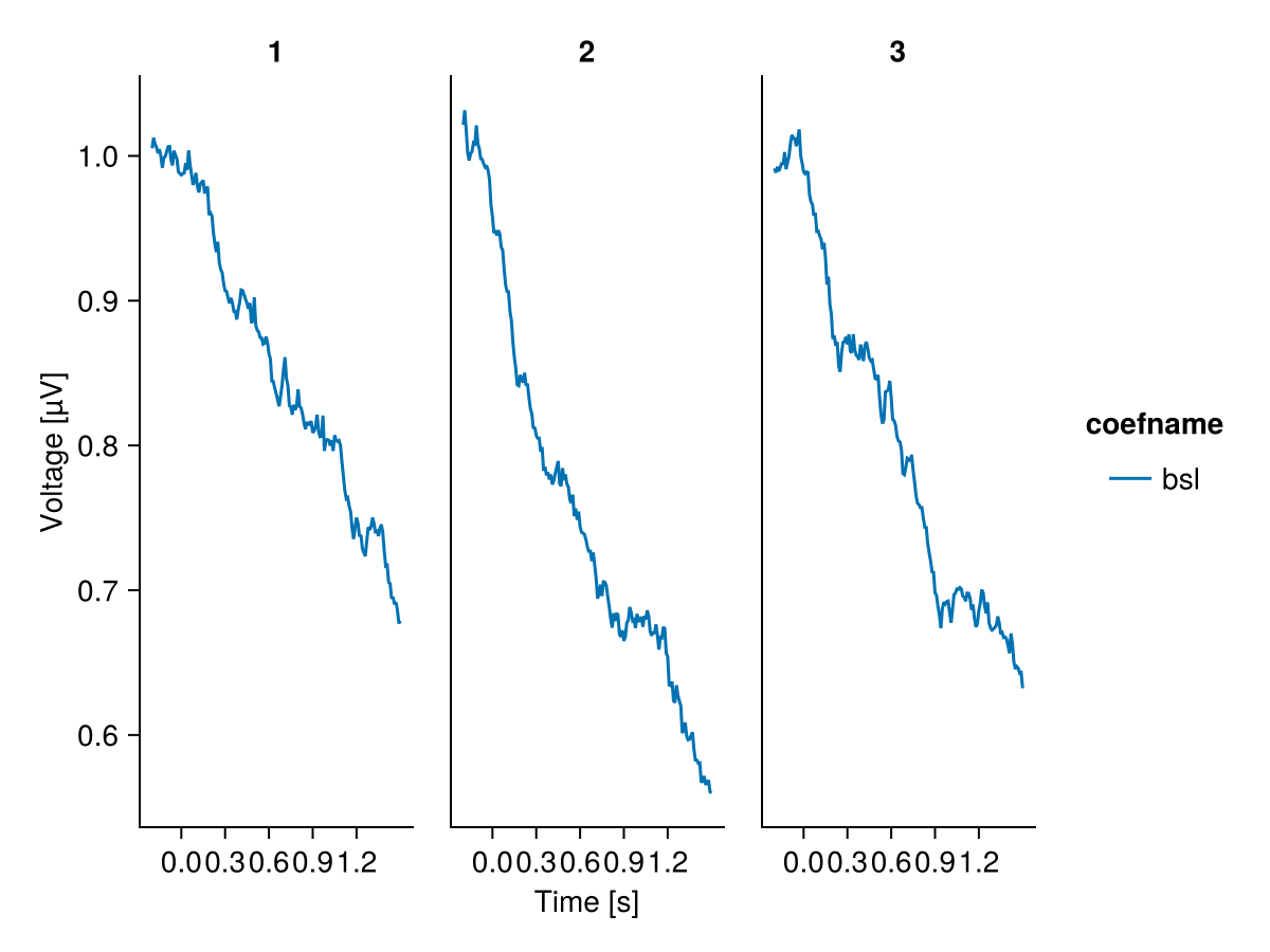
How to read this plot:
- Within the baseline window, the beta averages exactly 1 for every channel - by construction, the covariate is the window mean.
- Beyond the window, the beta decays with the drift's autocorrelation reach - to roughly 0.7 beyond 500 ms. A slow drift therefore co-varies with the entire epoch - the baseline is not just noise, and this plot makes its reach visible.
The baseline issue
What does this mean for the classical approach? We baseline-correct the same epochs (subtract the baseline mean) and fit a plain model:
data_corr = data_e .- mean(data_e[:, bsl_ix, :]; dims = 2)
f_plain = @formula 0 ~ 1 + condition
m_corr = fit(UnfoldLinearModel, [Any => (f_plain, times)], evts, data_corr)Unfold-Type: ::UnfoldLinearModel{Float64}
Any => 1 + condition
✔ model is fit. size(coefs) (3, 171, 2)
Useful functions: `design(uf)`, `designmatrix(uf)`, `coef(uf)`, `coeftable(uf)`Comparing the estimated condition effects: the conditions come in blocks, so each condition is seen against a different drift level - but with a stationary drift these differences average out over the trials of each block, and both approaches estimate similar effects. Neither removes the part of the drift the baseline cannot predict, late in the epoch - which is why baseline correction is no substitute for high-pass filtering. The difference between the methods is what they assume: correction fixes the baseline's influence at β = 1 at every latency, regression estimates it - and the coefficient plot above shows when that assumption holds.
ct_corr = coeftable(m_corr)
cmp = vcat(ct_corr, ct)
cmp.baseline = vcat(fill("correction", nrow(ct_corr)), fill("regression", nrow(ct)))
plot_erp(
    cmp[startswith.(cmp.coefname, "condition"), :];
    mapping = (; col = :channel, color = :baseline),
)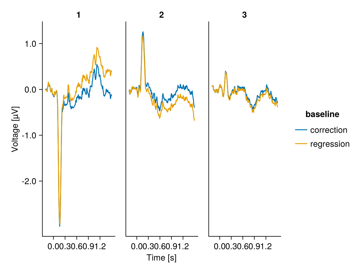
This is the baseline issue: whenever the baseline co-varies with the epoch, classical baseline correction subtracts signal along with the noise, and assumes its influence is β = 1 at every latency. Baseline regression instead estimates (and thereby removes) exactly this influence per channel - keeping the effects of interest conditional on the baseline.
This page was generated using Literate.jl.