Include multiple Visualizations in one Figure

This section discusses how users can incorporate multiple plots into a single figure.

Library load

using UnfoldMakie
using CairoMakie
using DataFramesMeta
using UnfoldSim
using Unfold
using MakieThemes
set_theme!(theme_ggthemr(:fresh)) # nicer defaults - should maybe be default?

Data input

include("../../../example_data.jl")
d_topo, positions = example_data("TopoPlots.jl")
uf_deconv = example_data("UnfoldLinearModelContinuousTime")
uf = example_data("UnfoldLinearModel")
results = coeftable(uf)
uf_5chan = example_data("UnfoldLinearModelMultiChannel")
data, positions = TopoPlots.example_data()
dat_e, evts, times = example_data("sort_data")
d_singletrial, _ = UnfoldSim.predef_eeg(; return_epoched = true)


#=
By using the !-version of the plotting function and inserting a grid position instead of an entire figure, we can create complex plot combining several figures.

We will start by creating a figure with `Makie.Figure`.

`f = Figure()`

Now any plot can be added to `f` by placing a grid position, such as `f[1, 1]`.
=#

f = Figure()
plot_erp!(f[1, 1], coeftable(uf_deconv))
plot_erp!(
    f[1, 2],
    effects(Dict(:condition => ["car", "face"]), uf_deconv),
    mapping = (; color = :condition),
)
plot_butterfly!(f[2, 1:2], d_topo; positions = positions)

f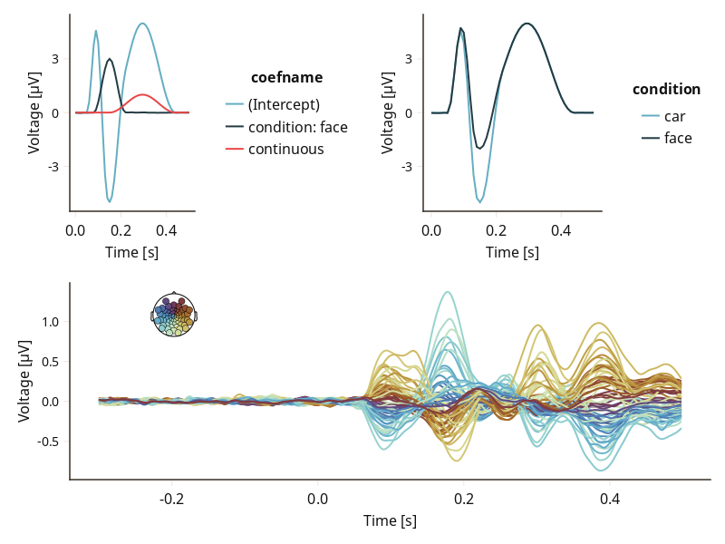

Very complex plot

Using the data from the tutorials, we can create a large image with any type of plot.

With so many plots at once, it's tempting to set a fixed resolution in your image to order the plots evenly (code below).

f = Figure(resolution = (2000, 2000))

plot_butterfly!(f[1, 1:3], d_topo; positions = positions)

pvals = DataFrame(
    from = [0.1, 0.15],
    to = [0.2, 0.5], # if coefname not specified, line should be black
    coefname = ["(Intercept)", "category: face"],
)
plot_erp!(
    f[2, 1:2],
    results,
    categorical_color = false,
    categorical_group = false,
    pvalue = pvals,
    stderror = true,
)

plot_designmatrix!(f[2, 3], designmatrix(uf))

plot_topoplot!(f[3, 1], data[:, 150, 1]; positions = positions)
plot_topoplotseries!(
    f[4, 1:3],
    d_topo,
    0.1;
    positions = positions,
    mapping = (; label = :channel),
)

res_effects = effects(Dict(:continuous => -5:0.5:5), uf_deconv)

plot_erp!(
    f[2, 4:5],
    res_effects;
    categorical_color = false,
    categorical_group = true,
    mapping = (; y = :yhat, color = :continuous, group = :continuous),
    legend = (; nbanks = 2),
    layout = (; show_legend = true, legend_position = :right),
)

plot_parallelcoordinates(
    f[3, 2:3],
    uf_5chan;
    mapping = (; color = :coefname),
    layout = (; legend_position = :right),
)

plot_erpimage!(f[1, 4:5], times, d_singletrial)
plot_circulareegtopoplot!(
    f[3:4, 4:5],
    d_topo[in.(d_topo.time, Ref(-0.3:0.1:0.5)), :];
    positions = positions,
    predictor = :time,
    predictor_bounds = [-0.3, 0.5],
)
f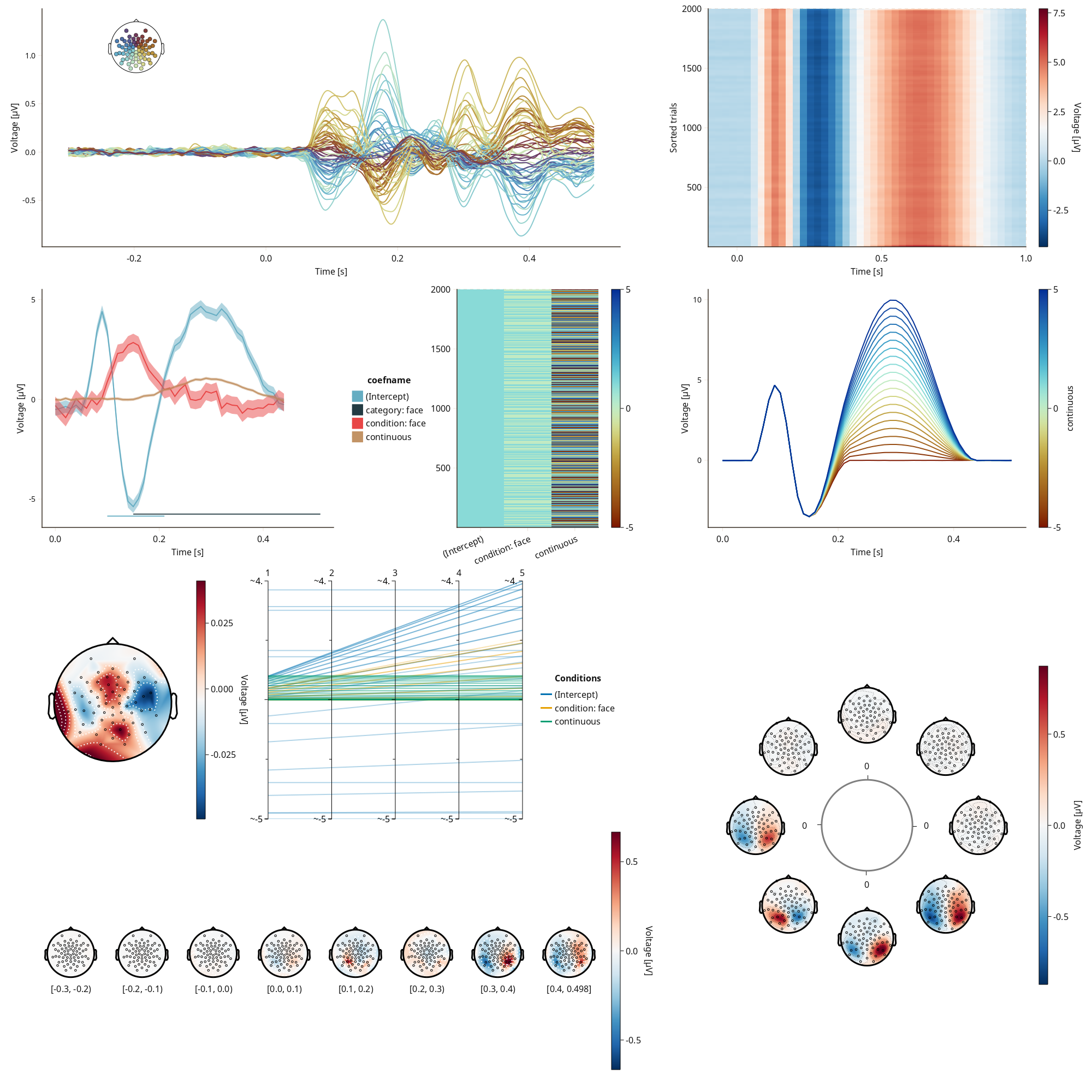

In two columns

f = Figure(resolution = (1200, 1400))
ga = f[1, 1]
gc = f[2, 1]
ge = f[3, 1]
gg = f[4, 1]
gb = f[1, 2]
gd = f[2, 2]
gf = f[3, 2]
gh = f[4, 2]

d_topo, pos = example_data("TopoPlots.jl")
data, positions = TopoPlots.example_data()
df = UnfoldMakie.eeg_matrix_to_dataframe(data[:, :, 1], string.(1:length(positions)))
raw_ch_names = [
    "FP1", "F3", "F7", "FC3", "C3", "C5", "P3", "P7", "P9", "PO7", "PO3", "O1",
    "Oz", "Pz", "CPz", "FP2", "Fz", "F4", "F8", "FC4", "FCz", "Cz",
    "C4", "C6", "P4", "P8", "P10", "PO8", "PO4", "O2",
]

m = example_data("UnfoldLinearModel")
results = coeftable(m)

results.coefname =
    replace(results.coefname, "condition: face" => "face", "(Intercept)" => "car")
results = filter(row -> row.coefname != "continuous", results)

plot_erp!(ga, results; :stderror => true, mapping = (; color = :coefname => "Conditions"))
hlines!(0, color = :gray, linewidth = 1)
vlines!(0, color = :gray, linewidth = 1)
plot_butterfly!(
    gb,
    d_topo;
    positions = pos,
    topomarkersize = 10,
    topoheigth = 0.4,
    topowidth = 0.4,
)
hlines!(0, color = :gray, linewidth = 1)
vlines!(0, color = :gray, linewidth = 1)
plot_topoplot!(gc, data[:, 340, 1]; positions = positions, axis = (; xlabel = "[340 ms]"))

plot_topoplotseries!(
    gd,
    df,
    80;
    positions = positions,
    visual = (label_scatter = false,),
    layout = (; use_colorbar = true),
)

ax = gd[1, 1] = Axis(f)
text!(ax, 0, 0, text = "Time [ms]", align = (:center, :center), offset = (-20, -80))
hidespines!(ax) # delete unnecessary spines (lines)
hidedecorations!(ax, label = false)

plot_erpgrid!(
    ge,
    data[:, :, 1],
    positions;
    axis = (; ylabel = "µV", ylim = [-0.05, 0.6], xlim = [-0.04, 1]),
)

dat_e, evts, times = example_data("sort_data")
plot_erpimage!(gf, times, dat_e; sortvalues = evts.Δlatency)
plot_channelimage!(gg, data[:, :, 1], positions[1:30], raw_ch_names;)
r1, positions = example_data()
r2 = deepcopy(r1)
r2.coefname .= "B" # create a second category
r2.estimate .+= rand(length(r2.estimate)) * 0.1
results_plot = vcat(r1, r2)
plot_parallelcoordinates(
    gh,
    subset(results_plot, :channel => x -> x .< 8, :time => x -> x .< 0);
    mapping = (; color = :coefname),
    normalize = :minmax,
    ax_labels = ["FP1", "F3", "F7", "FC3", "C3", "C5", "P3", "P7"],
)

for (label, layout) in
    zip(["A", "B", "C", "D", "E", "F", "G", "H"], [ga, gb, gc, gd, ge, gf, gg, gh])
    Label(
        layout[1, 1, TopLeft()],
        label,
        fontsize = 26,
        font = :bold,
        padding = (20, 20, 22, 0),
        halign = :right,
    )
end
f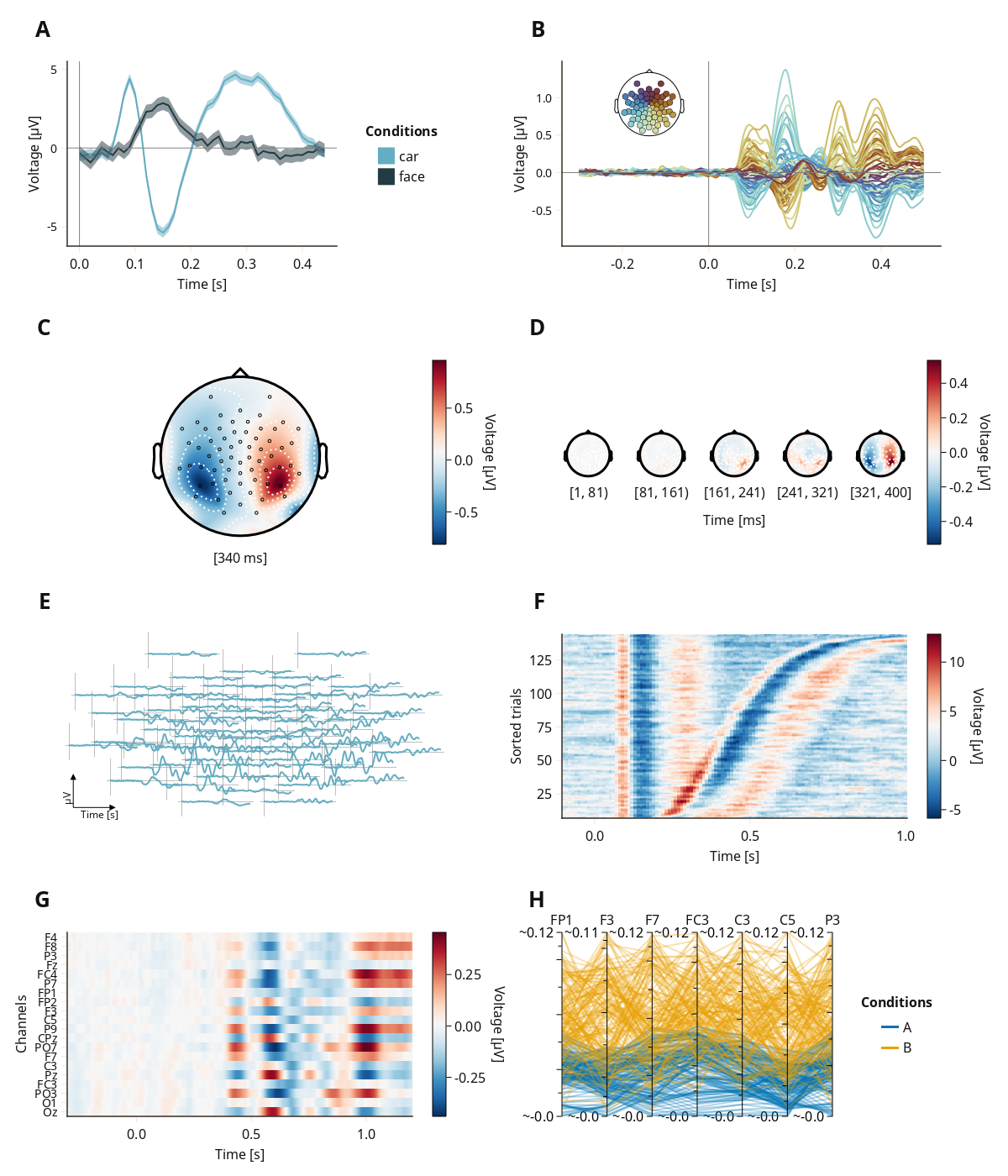

This page was generated using Literate.jl.