Speed measurement
Here we will compare the speed of plotting UnfoldMakie with MNE (Python) and EEGLAB (MATLAB).
Three cases are measured:
- Single topoplot
- Topoplot series with 50 topoplots
- Topoplott animation with 50 timestamps
Note that the results of benchmarking on your computer and on Github may differ.
using UnfoldMakie
using TopoPlots
using BenchmarkTools
using Observables
using CairoMakie
using Statistics
using PythonPlot;
using PyMNE;
CondaPkg Found dependencies: /home/runner/.julia/packages/CondaPkg/lKlVY/CondaPkg.toml
CondaPkg Found dependencies: /home/runner/.julia/packages/PyMNE/AlJE6/CondaPkg.toml
CondaPkg Found dependencies: /home/runner/.julia/packages/PythonCall/JksWe/CondaPkg.toml
CondaPkg Found dependencies: /home/runner/.julia/packages/PythonPlot/oS8x4/CondaPkg.toml
CondaPkg Dependencies already up to dateData input
dat, positions = TopoPlots.example_data()
df = UnfoldMakie.eeg_array_to_dataframe(dat[:, :, 1], string.(1:length(positions)));
Topoplots
UnfoldMakie.jl
@benchmark plot_topoplot(dat[:, 320, 1]; positions = positions)BenchmarkTools.Trial: 66 samples with 1 evaluation per sample.
Range (min … max): 43.556 ms … 1.484 s ┊ GC (min … max): 0.00% … 96.77%
Time (median): 44.952 ms ┊ GC (median): 0.00%
Time (mean ± σ): 76.185 ms ± 191.255 ms ┊ GC (mean ± σ): 40.42% ± 16.24%
█
█▁▁▁▁▁▁▁▁▁▁▁▁▁▁▁▁▁▁▁▁▁▁▁▁▁▁▁▁▁▁▁▁▁▁▁▁▁▁▁▁▁▁▁▁▁▁▁▁▁▁▁▁▁▁▁▁▁▁▄ ▁
43.6 ms Histogram: log(frequency) by time 654 ms <
Memory estimate: 11.82 MiB, allocs estimate: 194623.UnfoldMakie.jl with DelaunayMesh
@benchmark plot_topoplot(
    dat[:, 320, 1];
    positions = positions,
    topo_interpolation = (; interpolation = DelaunayMesh()),
)
BenchmarkTools.Trial: 69 samples with 1 evaluation per sample.
Range (min … max): 45.460 ms … 1.692 s ┊ GC (min … max): 0.00% … 96.82%
Time (median): 49.640 ms ┊ GC (median): 0.00%
Time (mean ± σ): 73.098 ms ± 197.808 ms ┊ GC (mean ± σ): 32.49% ± 11.66%
▁ ▄ █ ▁▁ ▄▁ ▄▄█ ▄█▁ ▁ ▁ ▄
▆▁▁▁▆▁▆▁▁█▆█▆█▁▆▆▁██▁▆██▆▁▆▁▁▆▁▆▆███▁▆███▆▁▆▁▆▆█▁▆▆█▁▁▆▁█▆▆▆ ▁
45.5 ms Histogram: frequency by time 52.8 ms <
Memory estimate: 11.82 MiB, allocs estimate: 194630.MNE
posmat = collect(reduce(hcat, [[p[1], p[2]] for p in positions])')
pypos = Py(posmat).to_numpy()
pydat = Py(dat[:, 320, 1])

@benchmark begin
    f = PythonPlot.figure()
    PyMNE.viz.plot_topomap(
        pydat,
        pypos,
        sphere = 1.1,
        extrapolate = "box",
        cmap = "RdBu_r",
        sensors = false,
        contours = 6,
    )
    f.show()
end
BenchmarkTools.Trial: 425 samples with 1 evaluation per sample.
Range (min … max): 10.784 ms … 202.077 ms ┊ GC (min … max): 0.00% … 0.00%
Time (median): 11.016 ms ┊ GC (median): 0.00%
Time (mean ± σ): 11.766 ms ± 9.547 ms ┊ GC (mean ± σ): 0.00% ± 0.00%
▄██▅▄
█████▇█▇▅▄▁▆▄▁▁▅▄▄▄▁▁▁▄▅▄▁▁▁▅▁▄▄▄▅▆▁▁▄▁▁▁▁▁▁▁▁▁▁▁▁▁▁▁▁▁▁▁▁▁▄ ▇
10.8 ms Histogram: log(frequency) by time 16.8 ms <
Memory estimate: 3.48 KiB, allocs estimate: 110.Topoplot series
Note that UnfoldMakie and MNE have different defaults for displaying topoplot series. UnfoldMakie in plot_topoplot averages over time samples. MNE in plot_topopmap displays single samples without averaging.
UnfoldMakie.jl
@benchmark begin
    plot_topoplotseries(
        df;
        bin_num = 50,
        positions = positions,
        axis = (; xlabel = "Time windows [s]"),
    )
end
BenchmarkTools.Trial: 3 samples with 1 evaluation per sample.
Range (min … max): 2.029 s … 3.300 s ┊ GC (min … max): 0.00% … 37.36%
Time (median): 2.202 s ┊ GC (median): 15.88%
Time (mean ± σ): 2.510 s ± 689.324 ms ┊ GC (mean ± σ): 21.02% ± 18.75%
█ █ █
█▁▁▁▁▁▁█▁▁▁▁▁▁▁▁▁▁▁▁▁▁▁▁▁▁▁▁▁▁▁▁▁▁▁▁▁▁▁▁▁▁▁▁▁▁▁▁▁▁▁▁▁▁▁▁▁█ ▁
2.03 s Histogram: frequency by time 3.3 s <
Memory estimate: 342.22 MiB, allocs estimate: 4921077.MNE
easycap_montage = PyMNE.channels.make_standard_montage("standard_1020")
ch_names = pyconvert(Vector{String}, easycap_montage.ch_names)[1:64]
info = PyMNE.create_info(PyList(ch_names), ch_types = "eeg", sfreq = 1)
info.set_montage(easycap_montage)
simulated_epochs = PyMNE.EvokedArray(Py(dat[:, :, 1]), info)

@benchmark simulated_epochs.plot_topomap(1:50)
BenchmarkTools.Trial: 9 samples with 1 evaluation per sample.
Range (min … max): 612.727 ms … 617.631 ms ┊ GC (min … max): 0.00% … 0.00%
Time (median): 613.629 ms ┊ GC (median): 0.00%
Time (mean ± σ): 613.958 ms ± 1.492 ms ┊ GC (mean ± σ): 0.00% ± 0.00%
█ ▁ ▁ ▁ █ ▁ ▁
█▁▁▁█▁▁▁█▁▁█▁▁█▁▁▁▁▁▁█▁▁▁▁▁▁▁▁▁▁▁▁▁▁▁▁▁▁▁▁▁▁▁▁▁▁▁▁▁▁▁▁▁▁▁▁▁▁█ ▁
613 ms Histogram: frequency by time 618 ms <
Memory estimate: 2.59 KiB, allocs estimate: 82.MATLAB
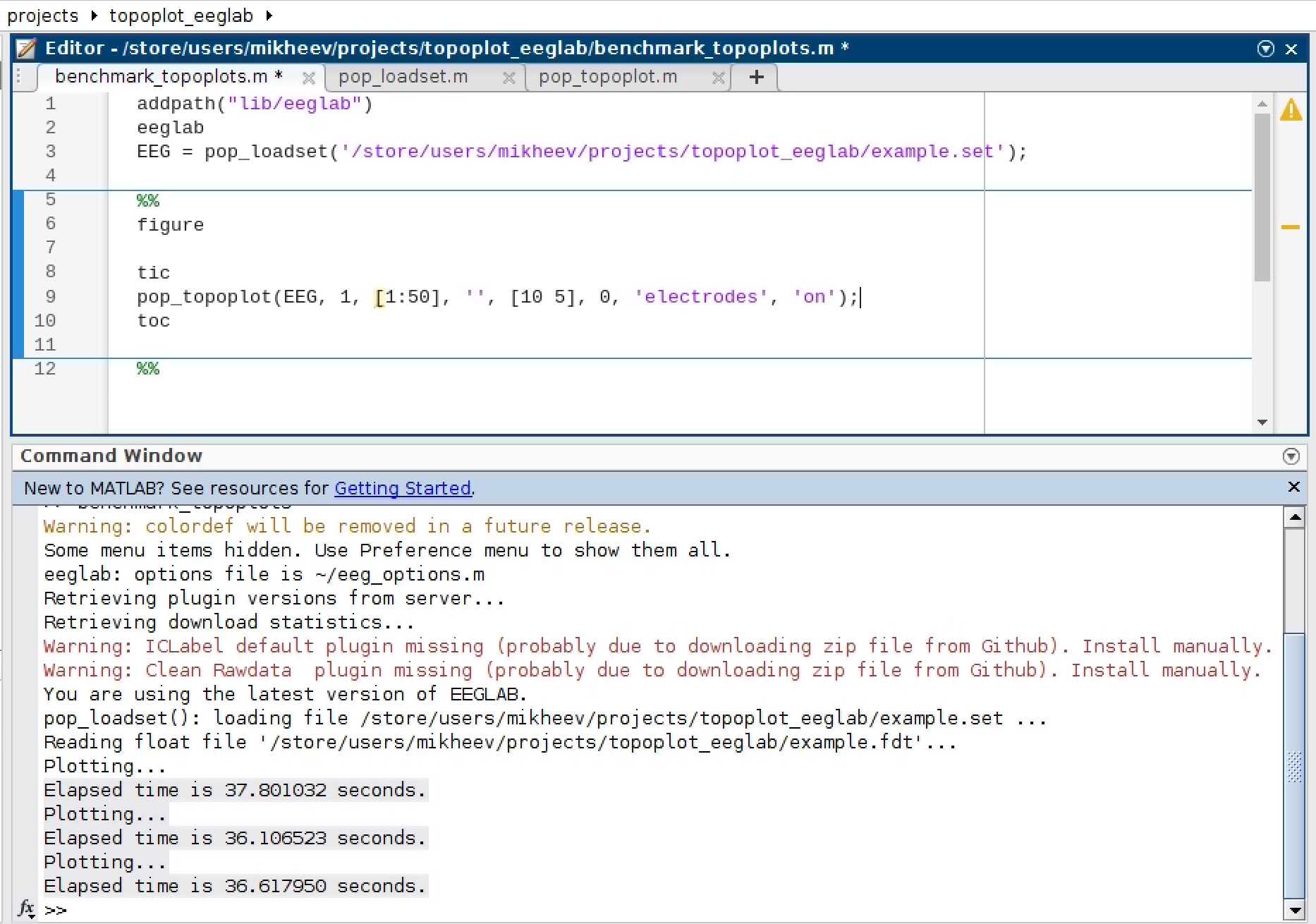
Running MATLAB on a GitHub Action is not easy. So we benchmarked three consecutive executions (on a screenshot) on a server with an AMD EPYC 7452 32-core processor. Note that Github and the server we used for MATLAB benchmarking are two different computers, which can give different timing results.
Animation
The main advantage of Julia is the speed with which the figures are updated.
timestamps = range(1, 50, step = 1)
framerate = 5050UnfoldMakie with .gif
vals = vec(dat[:, :, 1])
p01, p99 = quantile(vals, [0.01, 0.99])
m = max(abs(p01), abs(p99))
cr = Float32.((-m, m))
@benchmark begin
    f = Makie.Figure()
    dat_obs = Observable(dat[:, 1, 1])
    plot_topoplot!(f[1, 1], dat_obs, positions = positions, visual = (; contours = false, colorrange = cr),)
    record(f, "topoplot_animation_UM.gif", timestamps; framerate = framerate) do t
        dat_obs[] = @view(dat[:, t, 1])
    end
end
BenchmarkTools.Trial: 3 samples with 1 evaluation per sample.
Range (min … max): 2.168 s … 2.189 s ┊ GC (min … max): 1.93% … 2.25%
Time (median): 2.168 s ┊ GC (median): 1.93%
Time (mean ± σ): 2.175 s ± 12.213 ms ┊ GC (mean ± σ): 1.40% ± 1.22%
█ ▁
█▁▁▁▁▁▁▁▁▁▁▁▁▁▁▁▁▁▁▁▁▁▁▁▁▁▁▁▁▁▁▁▁▁▁▁▁▁▁▁▁▁▁▁▁▁▁▁▁▁▁▁▁▁▁▁█ ▁
2.17 s Histogram: frequency by time 2.19 s <
Memory estimate: 120.53 MiB, allocs estimate: 421087.
MNE with .gif
@benchmark begin
    fig, anim = simulated_epochs.animate_topomap(
        times = Py(timestamps),
        frame_rate = framerate,
        blit = false,
        image_interp = "cubic", # same as CloughTocher
    )
    anim.save("topomap_animation_mne.gif", writer = "ffmpeg", fps = framerate)
end
BenchmarkTools.Trial: 1 sample with 1 evaluation per sample.
Single result which took 7.340 s (0.00% GC) to evaluate,
with a memory estimate of 3.36 KiB, over 116 allocations.Note, that due to some bugs in (probably) PythonCall topoplot is black and white.
This page was generated using Literate.jl.