Complex figures
This section discusses how users can incorporate multiple plots into a single figure.
Setup
Library load
using UnfoldMakie;
using CairoMakie
using DataFrames
using UnfoldSim
using Unfold
using MakieThemes
using TopoPlots;
Data input
Click to expand
topo_df, positions = UnfoldMakie.example_data("TopoPlots.jl")
topo_array, _ = TopoPlots.example_data()
toposeries_data =
    UnfoldMakie.eeg_array_to_dataframe(topo_array[:, :, 1], string.(1:length(positions)));
biosemi32 = get_montage("biosemi32");
Exclude the three fiducial landmarks: Nz, LPA, and RPA.
biosemi32 = (; labels = biosemi32.labels[1:32], positions = biosemi32.positions[1:32]);

continuous_time_model = UnfoldMakie.example_data("UnfoldLinearModelContinuousTime")
linear_model = UnfoldMakie.example_data("UnfoldLinearModel");
multichannel_model = UnfoldMakie.example_data("UnfoldLinearModelMultiChannel");

erpimage_data, events, time_points = UnfoldMakie.example_data("sort_data")
epoched_data, _ = UnfoldSim.predef_eeg(; return_epoched = true);

coefficient_table = coeftable(linear_model);
coefficient_table.coefname =
    replace(coefficient_table.coefname, "condition: face" => "face", "(Intercept)" => "car");
coefficient_table = filter(row -> row.coefname != "continuous", coefficient_table);

circular_topo_data = DataFrame(
    :estimate => eachcol(Float64.(topo_array[:, 100:40:300, 1])),
    :circular_variable => [0, 50, 80, 120, 180, 210],
    :time => 100:40:300,
);
circular_topo_data = flatten(circular_topo_data, :estimate);
Basic complex figure
By using the !-version of the plotting function and inserting a grid position instead of an entire figure, we can create complex plot that combines several figures. We will start by creating a figure with Makie.Figure.
Now any plot can be added to f by placing a grid position, such as f[1, 1]. Also we used a specified theme fresh.
f = Figure(size = (750, 500))
with_theme(theme_ggthemr(:fresh)) do
    plot_erp!(
        f[1, 1],
        coeftable(continuous_time_model);
        mapping = (; color = :coefname => "Conditions"),
    )
    plot_erp!(
        f[1, 2],
        effects(Dict(:condition => ["car", "face"]), continuous_time_model),
        mapping = (; y = :yhat, color = :condition => "Conditions"),
    )
    plot_butterfly!(f[2, 1:2], topo_df; positions = positions,
        topo_attributes = (; label_scatter = (; markersize = 5)),
        topo_axis = (; height = Relative(0.5), width = Relative(0.5)))
end
f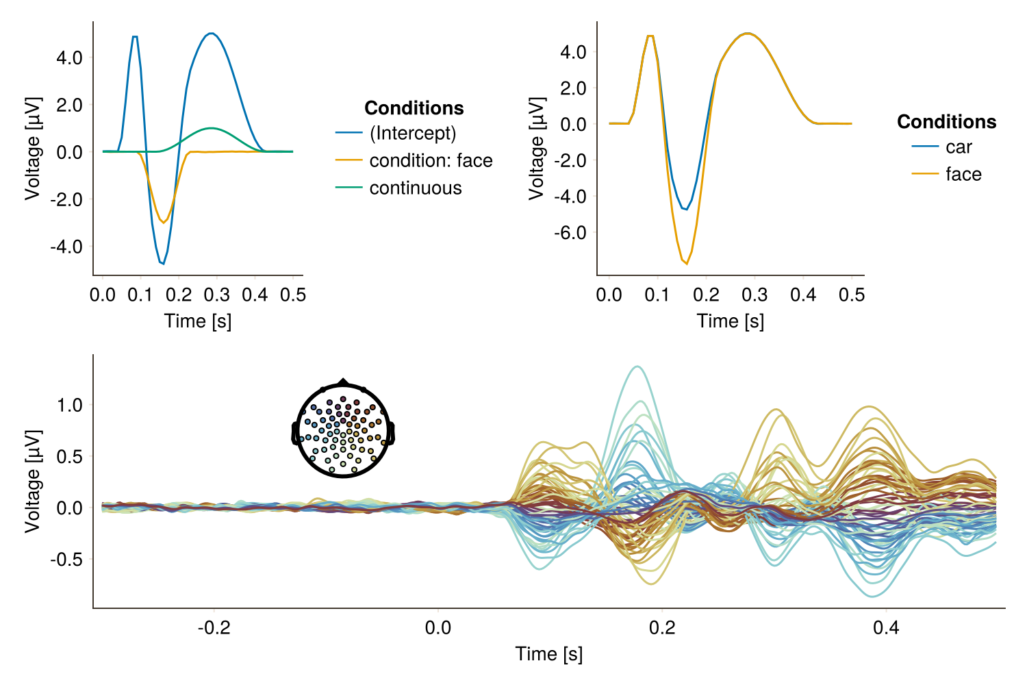
A very complex figure
We can create a large figure with any type of plot using predefined data.
With so many plots at once, it's better to set a fixed resolution in your image to arrange the plots evenly.
Click to expand
begin
    f = Figure(size = (2000, 2000))

    plot_butterfly!(f[1, 1:3], topo_df; positions = positions)

    pvals = DataFrame(
        from = [0.1, 0.15],
        to = [0.2, 0.5], # if coefname not specified, line should be black
        coefname = ["(Intercept)", "category: face"],
    )
    plot_erp!(f[2, 1:2], coefficient_table, significance = pvals, stderror = true)

    plot_designmatrix!(f[2, 3], designmatrix(linear_model))

    plot_topoplot!(f[3, 1], topo_array[:, 150, 1]; positions = positions)
    plot_topoplotseries!(
        f[4, 1:3],
        topo_df;
        bin_width = 0.1,
        positions = positions,
        mapping = (; label = :channel),
    )

    res_effects = effects(Dict(:continuous => -5:0.5:5), continuous_time_model)

    plot_erp!(
        f[2, 4:5],
        res_effects;
        mapping = (; y = :yhat, color = :continuous, group = :continuous => nonnumeric),
        legend = (; nbanks = 2),
    )

    plot_parallelcoordinates(
        f[3, 2:3],
        multichannel_model;
        mapping = (; color = :coefname),
    )

    plot_erpimage!(f[1, 4:5], time_points, epoched_data)
    plot_circular_topoplots!(
        f[3:4, 4:5],
        topo_df[in.(topo_df.time, Ref(-0.3:0.1:0.5)), :];
        positions = positions,
        predictor = :time,
        predictor_bounds = [-0.3, 0.5],
    )
end
GridPosition(GridLayout[4, 5] (9 children), GridLayoutBase.Span(3:4, 4:5), GridLayoutBase.Inner())f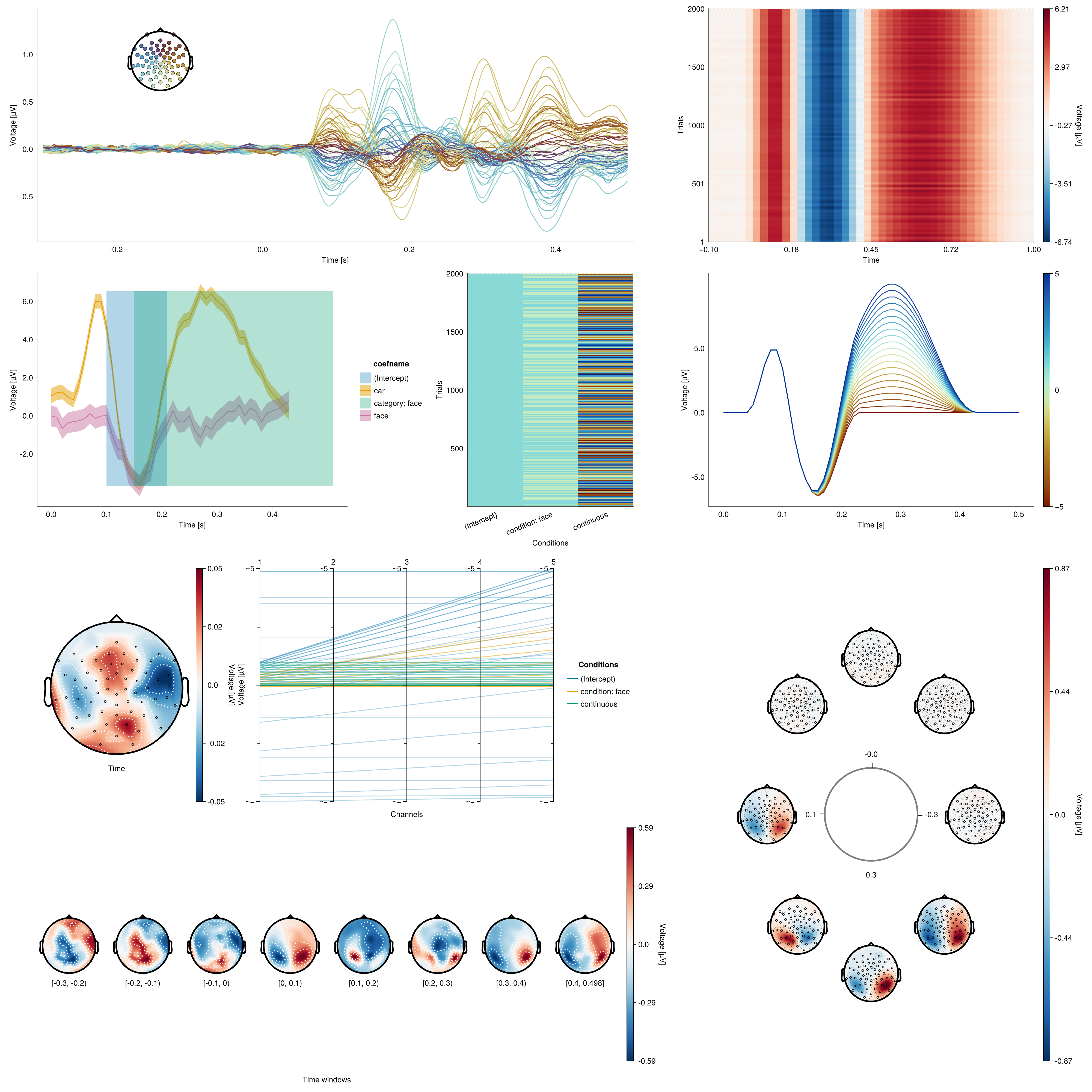
Complex figure in two columns and with background color
Click to expand
function complex_figure3(
    topo_df,
    topo_array,
    positions,
    toposeries_data,
    biosemi32,
    coefficient_table,
    circular_topo_data,
    erpimage_data,
    events,
    time_points,
)
    f = Figure(size = (1200, 1700))
    (panel_a, panel_c, panel_e, panel_g, panel_i) =
        (f[1, 1], f[2, 1], f[3, 1], f[4, 1], f[5:6, 1])
    (panel_b, panel_d, panel_f, panel_h, panel_j) =
        (f[1, 2], f[2, 2], f[3, 2], f[4, 2], f[5:6, 2])

    plot_erp!(
        panel_a,
        coefficient_table;
        stderror = true,
        mapping = (; color = :coefname => "Conditions"),
        axis = (; backgroundcolor = colorant"#F4F3EF", xlabel = "Time [ms]"),
    )
    hlines!(0, color = :gray, linewidth = 1)
    vlines!(0, color = :gray, linewidth = 1)
    plot_butterfly!(
        panel_b,
        topo_df;
        positions = positions,
        topo_axis = (; height = Relative(0.4), width = Relative(0.4)),
        axis = (; backgroundcolor = colorant"#F4F3EF", xlabel = "Time [ms]"),
    )
    hlines!(0, color = :gray, linewidth = 1)
    vlines!(0, color = :gray, linewidth = 1)
    plot_topoplot!(
        panel_c,
        topo_array[:, 340, 1];
        positions = positions,
        topo_axis = (; backgroundcolor = colorant"#F4F3EF"),
        axis = (; xlabel = "[340 ms]"),
    )

    plot_topoplotseries!(
        panel_d,
        toposeries_data;
        bin_width = 80,
        positions = positions,
        visual = (label_scatter = false, contours = false),
        layout = (; use_colorbar = true),
        topo_axis = (; backgroundcolor = colorant"#F4F3EF"),
        axis = (; backgroundcolor = colorant"#F4F3EF", xlabel = "Time [ms]"),
    )

    plot_erpgrid!(
        panel_e,
        topo_array[:, :, 1],
        positions;
        indicator_grid_axis = (;
            ylim = [-0.05, 0.6], xlim = [-0.04, 1], text_x_kwargs = (; text = "s"),
            text_y_kwargs = (; text = "µV"),
        ),
        axis = (; backgroundcolor = colorant"#F4F3EF",),
    )

    plot_erpimage!(
        panel_f,
        time_points,
        erpimage_data;
        sortvalues = events.Δlatency,
        axis = (; xlabel = "Time [ms]"),
    )
    spline_model = UnfoldMakie.example_data("UnfoldLinearModelwith1Spline")
    plot_splines!(
        panel_g,
        spline_model;
        spline_axis = (; backgroundcolor = colorant"#F4F3EF"),
        density_axis = (; backgroundcolor = colorant"#F4F3EF"),
    )

    parallel_df = subset(topo_df, :channel => x -> x .< 8, :time => x -> x .< 0)
    parallel_df_b = copy(parallel_df)
    parallel_df_b.coefname .= "B"
    parallel_df_b.estimate .+= 0.1
    parallel_df = vcat(parallel_df, parallel_df_b)
    plot_parallelcoordinates(
        panel_h,
        parallel_df;
        mapping = (; color = :coefname),
        normalize = :minmax,
        ax_labels = ["FP1", "F3", "F7", "FC3", "C3", "C5", "P3", "P7"],
        axis = (; backgroundcolor = colorant"#F4F3EF", ylabel = "Time [ms]"),
    )

    plot_circular_topoplots!(
        panel_i,
        circular_topo_data;
        positions = positions,
        center_label = "Time [s]",
        predictor = :time,
        topo_attributes = (; label_scatter = false,),
        topo_axis = (; backgroundcolor = colorant"#F4F3EF"),
        axis = (; backgroundcolor = colorant"#F4F3EF"),
        predictor_bounds = [80, 320],
        colorbar = (; height = 180),
    )
    plot_channelimage!(
        panel_j,
        topo_array[1:32, :, 1],
        biosemi32.positions,
        biosemi32.labels;
        axis = (; xlabel = "Time [ms]"),
    )

    for (label, layout) in
        zip(
        ["A", "B", "C", "D", "E", "F", "G", "H", "I", "J"],
        [panel_a, panel_b, panel_c, panel_d, panel_e,
        panel_f, panel_g, panel_h, panel_i, panel_j],
    )
        Label(
            layout[1, 1, TopLeft()],
            label,
            fontsize = 26,
            font = :bold,
            padding = (20, 20, 22, 0),
            halign = :right,
        )
    end
    f
end
complex_figure3 (generic function with 1 method)with_theme(Theme(; backgroundcolor = colorant"#F4F3EF")) do
complex_figure3(
topo_df,
topo_array,
positions,
toposeries_data,
biosemi32,
coefficient_table,
circular_topo_data,
erpimage_data,
events,
time_points,
)
end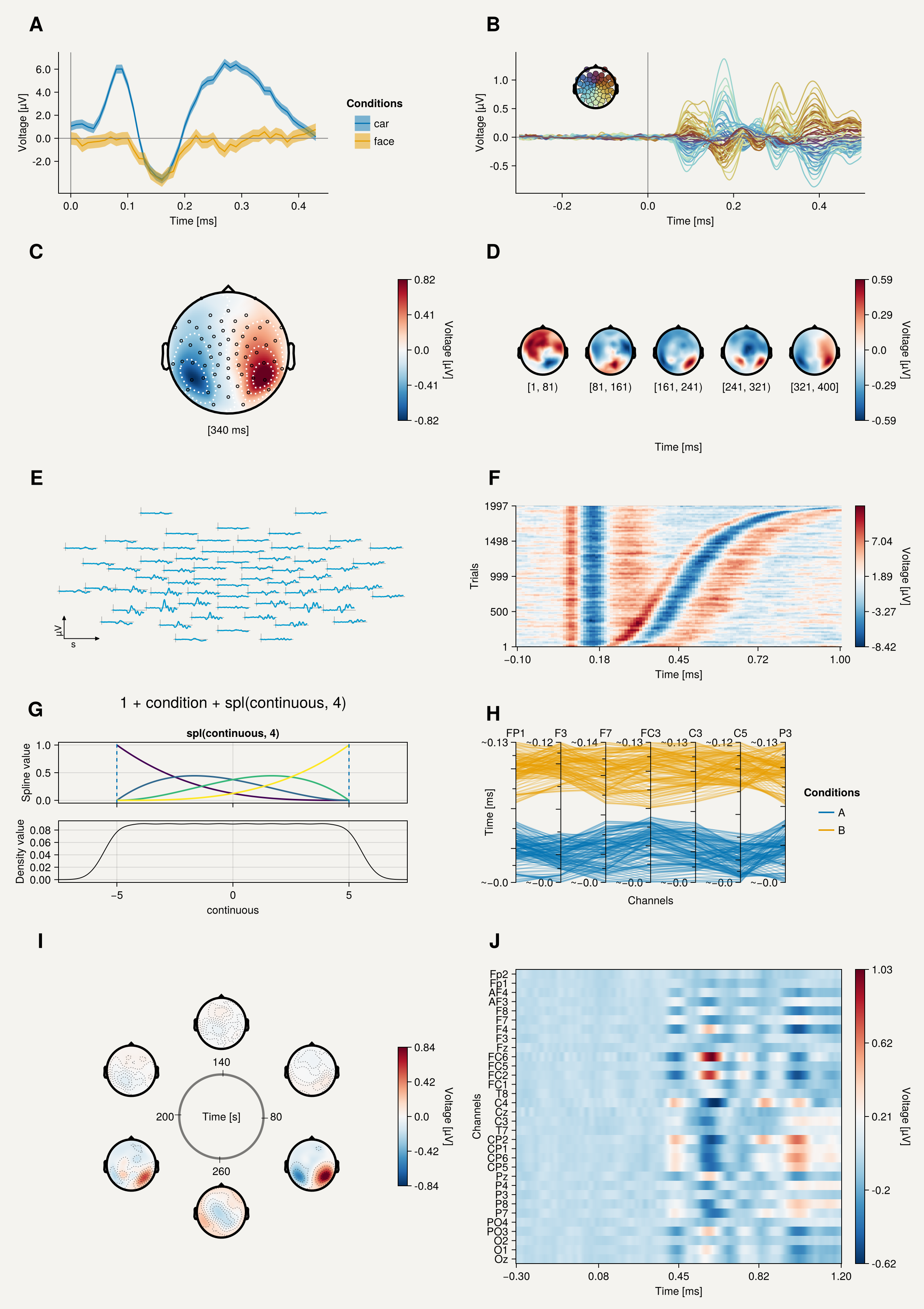
Complex figure in four columns and with background color
Click to expand
function complex_figure4(
    topo_df,
    topo_array,
    positions,
    toposeries_data,
    biosemi32,
    coefficient_table,
    circular_topo_data,
    erpimage_data,
    events,
    time_points,
)
    f = Figure(size = (1800, 1000))
    panel_background = colorant"#F4F3EF"
    axis_fontsizes =
        (; xlabelsize = 24, ylabelsize = 24, xticklabelsize = 18, yticklabelsize = 18)
    colorbar_style = (; labelsize = 24, ticklabelsize = 18)

    top_row = f[1, 1] = GridLayout()
    bottom_row = f[2, 1] = GridLayout()

    (panel_a, panel_b, panel_c, panel_d) =
        (top_row[1, 1], top_row[1, 2], top_row[1, 3], top_row[1, 4])
    (panel_e, panel_f, panel_h) =
        (bottom_row[1, 1], bottom_row[1, 2], bottom_row[1, 4])
    panel_g = bottom_row[1, 3] = GridLayout()

    plot_erp!(
        panel_a,
        coefficient_table;
        :stderror => true,
        mapping = (; color = :coefname => "Conditions:"),
        legend = (;
            orientation = :horizontal,
            titleposition = :left,
            position = :bottom,
            labelsize = 18,
            titlesize = 20,
            nbanks = 2,
        ),
        axis = (;
            axis_fontsizes...,
            backgroundcolor = panel_background,
            xlabel = "Time [ms]",
            width = 350,
        ),
    )
    hlines!(0, color = :gray, linewidth = 1)
    vlines!(0, color = :gray, linewidth = 1)

    plot_butterfly!(
        panel_b,
        topo_df;
        positions = positions,
        topo_axis = (;
            height = Relative(0.4),
            width = Relative(0.4),
            tellwidth = false,
            tellheight = false,
        ),
        axis = (; axis_fontsizes..., backgroundcolor = panel_background, xlabel = "Time [ms]"),
    )
    hlines!(0, color = :gray, linewidth = 1)
    vlines!(0, color = :gray, linewidth = 1)

    panel_e_objects = plot_topoplot!(
        panel_e,
        topo_array[:, 340, 1];
        positions = positions,
        return_objects = true,
        topo_axis = (; backgroundcolor = panel_background),
        axis = (;
            xlabel = "[340 ms]",
            backgroundcolor = panel_background,
            xlabelsize = 24,
            ylabelsize = 24,
        ),
        colorbar = (; colorbar_style..., position = :bottom, vertical = false, width = 240),
        visual = (; contours = false),
    )
    translate!(panel_e_objects.colorbar.blockscene, 0, -30, 100)

    plot_topoplotseries!(
        panel_f,
        toposeries_data;
        bin_num = 4,
        nrows = 2,
        positions = positions,
        visual = (label_scatter = false, contours = false),
        layout = (; use_colorbar = true),
        topo_axis = (; backgroundcolor = panel_background, xlabelsize = 18),
        axis = (;
            xlabelpadding = 50,
            backgroundcolor = panel_background,
            xlabel = "        Time [ms]",
            xlabelsize = 24,
            ylabelsize = 24,
        ),
        colorbar = (; colorbar_style..., height = 180),
    )

    plot_erpgrid!(
        panel_c,
        topo_array[:, :, 1],
        positions;
        indicator_grid_axis = (;
            ylim = [-0.05, 0.6], xlim = [-0.07, 1],
            text_x_kwargs = (; text = "s", fontsize = 24),
            text_y_kwargs = (; text = "µV", fontsize = 24),
        ),
        axis = (; backgroundcolor = panel_background),
        colorbar = (; colorbar_style..., height = 180),
    )

    plot_erpimage!(
        panel_d,
        time_points,
        erpimage_data;
        sortvalues = events.Δlatency,
        axis = (;
            axis_fontsizes...,
            xlabel = "Time [ms]",
        ),
        colorbar = (; colorbar_style..., height = 180),
    )

    panel_g_objects = plot_circular_topoplots!(
        panel_g,
        circular_topo_data;
        positions = positions,
        return_objects = true,
        center_label = "Time [ms]",
        predictor = :time,
        plot_radius = 0.9,
        topo_attributes = (; label_scatter = false, contours = false),
        topo_axis = (;
            backgroundcolor = panel_background,
            width = Relative(0.3),
            height = Relative(0.3),
        ),
        axis = (; backgroundcolor = panel_background, xlabelsize = 24, ylabelsize = 24),
        predictor_bounds = [80, 320],
        colorbar = (;
            position = :bottom,
            vertical = false,
            valign = :bottom,
            colorbar_style...,
            width = 240,
        ),
    )
    translate!(panel_g_objects.colorbar.blockscene, 0, -30, 100)
    colsize!(panel_g, 1, Relative(1))
    rowsize!(panel_g, 1, Relative(0.99))
    rowgap!(panel_g, 5)

    plot_channelimage!(
        panel_h,
        topo_array[1:32, :, 1],
        biosemi32.positions,
        biosemi32.labels;
        axis = (;
            axis_fontsizes...,
            xlabel = "Time [ms]",
        ),
        colorbar = (; colorbar_style..., height = 180),
    )

    for row_layout in (top_row, bottom_row), column = 1:4
        colsize!(row_layout, column, Relative(1 / 4))
    end

    for (label, layout) in zip(
        ["A", "B", "C", "D", "E", "F", "G", "H"],
        [panel_a, panel_b, panel_c, panel_d, panel_e, panel_f, panel_g, panel_h],
    )
        Label(
            layout[1, 1, Top()],
            label,
            fontsize = 26,
            font = :bold,
            padding = (20, 20, 22, 0),
            halign = :left,
        )
    end
    f
end
complex_figure4 (generic function with 1 method)f = with_theme(Theme(; backgroundcolor = colorant"#F4F3EF")) do
complex_figure4(
topo_df,
topo_array,
positions,
toposeries_data,
biosemi32,
coefficient_table,
circular_topo_data,
erpimage_data,
events,
time_points,
)
end
#save("complex_figure4.png", f)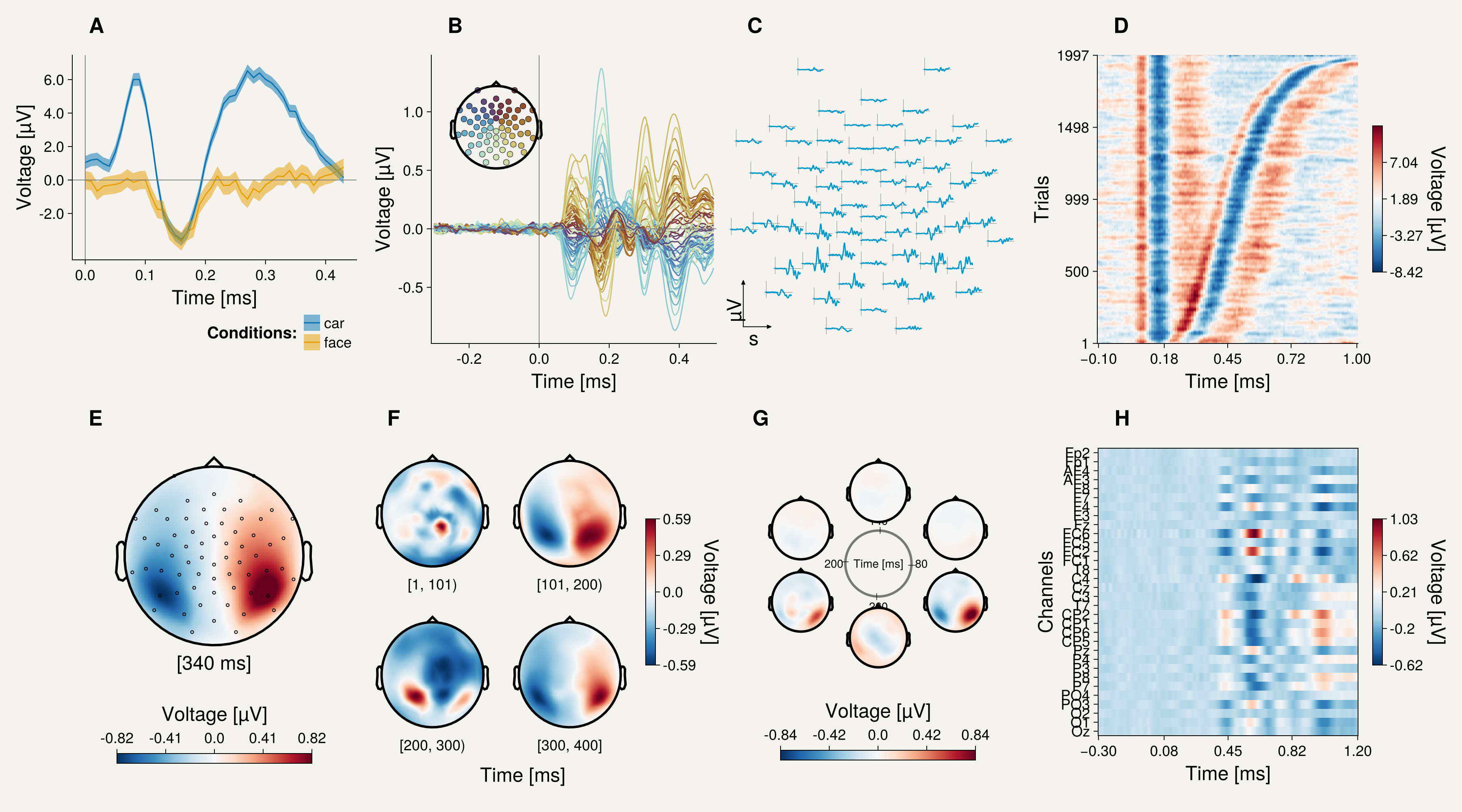
This page was generated using Literate.jl.